Pandas in action “how to automate your data analysis process”

If you are going down this rabbit hole of becoming a data scientist, regardless of whether you started a week ago or 10 years back, you know that it feels pretty much like riding a bike, but the bike is on fire, you are on fire, and the whole place is on fire.

Now, let’s say that you want to avoid riding the bike but you are seeking to have some sense of how to deal with data using the libraries available for this purpose without requiring a ton of your cycles to get started.

The good news is that there are hundreds of different open source tools that can help you to easily navigate through data and obtain outstanding results without being a pro.

For this purpose, we will use Python along with some other libraries. As you know, Python is the most popular language for data science out there, so I recommend you to get familiar with this programming language. Nevertheless, the goal of this post is to give you everything you need to start working with data without being a data scientist or a python programmer.

What is all this Pandas about?

Pandas is a python library for data analysis. Pandas is a toolbox for data manipulation operations such as sorting, filtering, cleaning, aggregating, pivoting, and more. If you have some experience with Microsoft Excel, this may sound familiar to you, right?

Pandas is comparable to Microsoft’s Excel and Google’s Sheets application. In all three technologies, a user interacts with tables consisting of rows and columns of data.

The technological ecosystem of tools for working with data has grown tremendously regardless of the programming language or framework of your choice, and Pandas is one of the most popular solutions available for data analysis and manipulation that you will use as part of your activities as a data scientist.

Pandas require a different mindset when compared to a traditional graphical spreadsheet. Programming is definitely more verbal than it is visual. We communicate with the software through instructions (programming functions and methods). You need to send the correct instructions, parameters, and orders to receive the expected output.

Pandas have a different learning curve. But, you shouldn't worry, if you have run functions such as SUMIF, VLOOKUP, or HLOOKUPin Excel or Google spreadsheet, you already sent instructions to the application as a real programmer.

Our first steps with Pandas

As I mentioned previously, the intention of this post is to give you the tools to manage data like a data scientist without being a hardcore programmer. If you are looking for in-depth content on Pandas, I recommend Pandas in Action.

Pandas include a number of methods to create and manage indexes, sort data, or even pivot between columns and rows.

For the purpose of the different examples, we will use Google Colab as our notebook, load data from files, and run some basic operations, similar to what you would do in Microsoft’s Excel. We will do some magic with another tool, bear with me for a few minutes.

Let's begin. Open a new notebook in Colab and lets import Pandas Library.

import pandas as pd

Easy, right?

Now, before we move forward, let’s introduce the concept of a Dataframe.

Think of a Dataframe as an object, a container for data. Different objects are optimized for different types of data, and we interact with them in different ways. Pandas use Dataframes to store multicolumn data sets. A DataFrame is comparable to a multicolumn table in Excel.

With that said, let’s load some data into a Dataframe.

That’s it! Ok. You may be thinking, can you break it down? Sure!

Python, as any other programming language, handles multiple types of data, int, float, char, strings, etc. Yeap, Boring, I know. But, something interesting about Python is how easy you can to assign data to variables without worrying about data type specification.

For example:

a = 5

Here we assign the value (type int) 5 to the variable a.

Another example would be:

my_name = 'Pikachu'

If we print the my_name variable we will see the following result:

print(my_name)

So far so good, right? now, remember our first example?

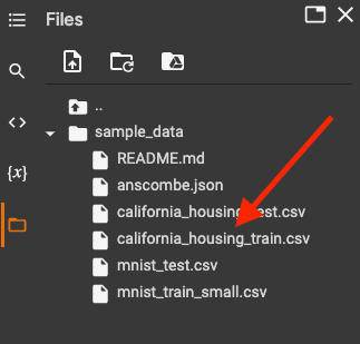
import pandas as pddf = pd.read_csv('./sample_data/california_housing_train.csv')

Here, we are using Pandas’ method read_csv to load a CSV file into a dataframe known as df. (We are referencing Pandas library via the pd alias). Finally, the CSV that we are loading, is a sample file spun up with your Colab Notebook. You can find it by navigating the files structure in Colab’s left panel. (If you are using another IDE, You should upload the data first)

Now, if we print the dataframe or just call it by its name:

df

We will see the following output.

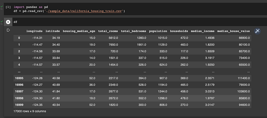
With two simple lines, you have loaded a CSV file into a Dataframe. Now, you can start exploring and transforming data.

Exploring a dataset

With Pandas and our mighty friend Python, you can run some easy instructions to explore and transform data as you wish.

Let’s say that you want to get the first 10 rows of your dataframe.

df.head(10)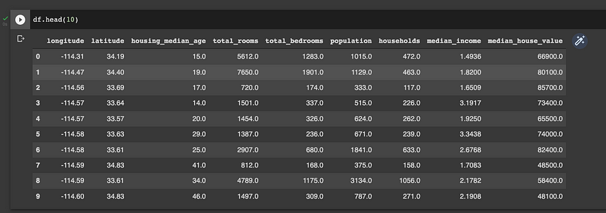

or vice versa, the last 10

df.tail(10)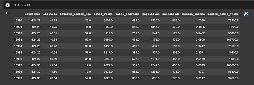

What about if you want to sort the data by its median_house_value attribute?

df.sort_values(by='median_house_value')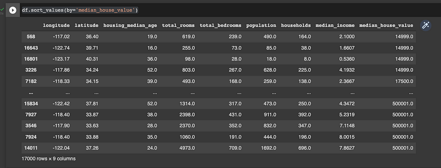

Now, when you combine the power of Pandas with Python, you can get some cool stuff. What about if we run the same command, but with a twist, I only want the first 10 rows of the sorted dataframe?
You can use methods and combine them to explore and transform the data as you need.

df.sort_values(by='median_house_value').head(10)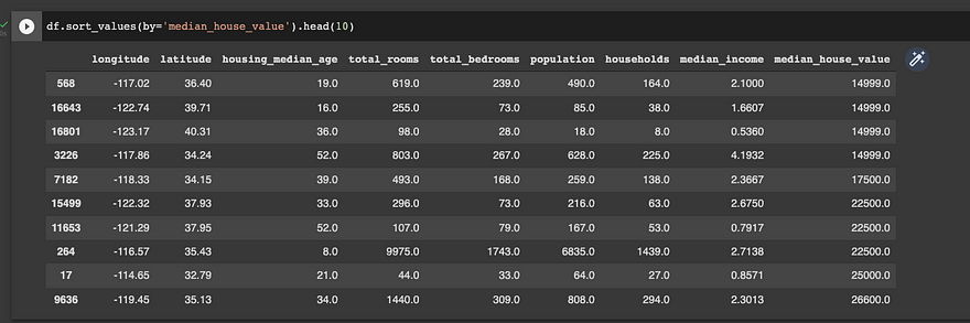

Index

The index is the range of ascending numbers that you can see on the left side of the DataFrame. You can think of them as the row number that you have in Microsoft Excel. You can alter those indexes and add labels as identifiers. You can use columns as the index of a DataFrame, but if not defined Pandas generates a numeric index starting from 0 by default as shown in the examples above. For this particular dataset we don’t have a good candidate for a single row label, but let’s imagine that we want to use longitude and latitude attributes as identifiers. You can accomplish this task by using the set_index method and storing the result into a new variable that we’ll call df_with_index. Why we are doing this? because you need to keep in mind that the original Dataframe won’t change unless you override its value, and it’s a good practice to create “new instances” of your Dataframes as you move forward with your data analysis.

df_with_index = df.set_index(['longitude','latitude'])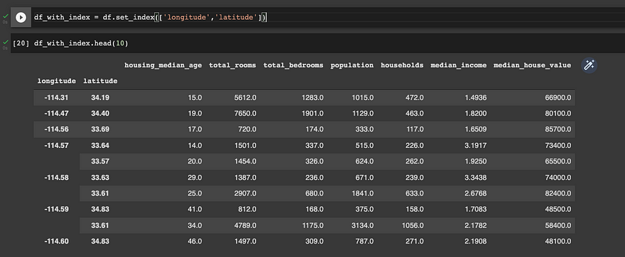

With one simple line, you have modified your Dataframe to use these two attributes as rows identifiers.

You may be wondering, Why do I need this? Let’s picture this. Your boss originally sent you the Dataset as a CSV file, and now she needs the data only of a particular longitude value.

You can use the Loc method and find all the entries that match for specific row identifier. For example, let’s grab all the entries for longitude value -114.57

df_with_index.loc[-114.57]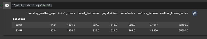

As you can see we have only two entries with different latitude values. Cool, right?

There is another option for when you don’t have an index defined. We can extract a row from the data set by its numeric order in line. You can use the method .iloc along with the row number to find what you need. In most programming languages, the index starts counting at 0.

df.iloc[0]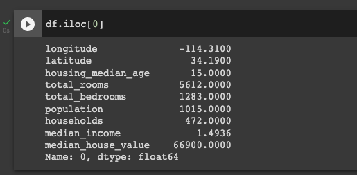

Pivoting with data

A pivot table is a data summary tool often found in spreadsheet programs. Aggregates a table of data by one or more keys, arranging the data in a rectangle with some of the group keys along the rows and some along with the columns.

Pivot tables in Python with pandas are possible through the groupby function. DataFrame has a pivot_table method and there is also a top-level pandas.pivot_table function. In addition to providing a convenient interface for groupby, pivot_table can add partial totals, also known as margins.

Following our example, let’s imagine that your boss is asking for a report with the median_house_value and median_income columns mean grouped by the longitude and latitude attributes. You can accomplish this by using the pivot_table method.

df_pivot_table = df.pivot_table(['median_house_value',
'median_income'], index=['longitude','latitude'])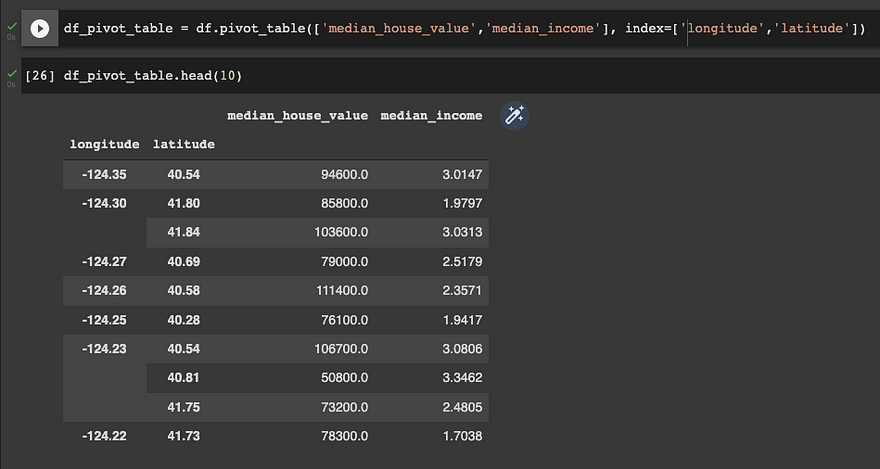

With one line you have created a report that shows the median income per median house value, grouped by longitude and latitude. That’s quite cool, isn’t it?

If you want to get deep into Pandas, please refer to Pandas Docs Library. Here you will find all the commands and methods required to boost your data analysis process.

Lets the magic begins

Pandas is definitely the best tool for data analysis in Python, but, let’s be honest, the transition between Microsoft Excel to Python is challenging for those with little coding experience.

What about if you have a tool that can help you to work with Pandas as if you were using Microsoft Excel or Google Spreadsheets?

In this section, we will discuss how to create pivot tables, join tables, filter data, and more using a Python library that allows us to work with a Pandas dataframe using an Excel GUI alike and automatically generates Pandas code for us.

For the purpose of this lab, we will use Mito Sheet.

Mito Sheet installation

Regardless of the IDE of your choice, you must install Mito Sheet and we will use Jupyter notebook rather than Colab. Don’t worry, Jupyter is as user-friendly as Colab and offers many benefits compared to other applications out there.

The following steps can be run on any operating system as long as you have a proper Python environment set up. First, download the package:

python -m pip install mitoinstaller

And, next, run the installer.

python -m mitoinstaller install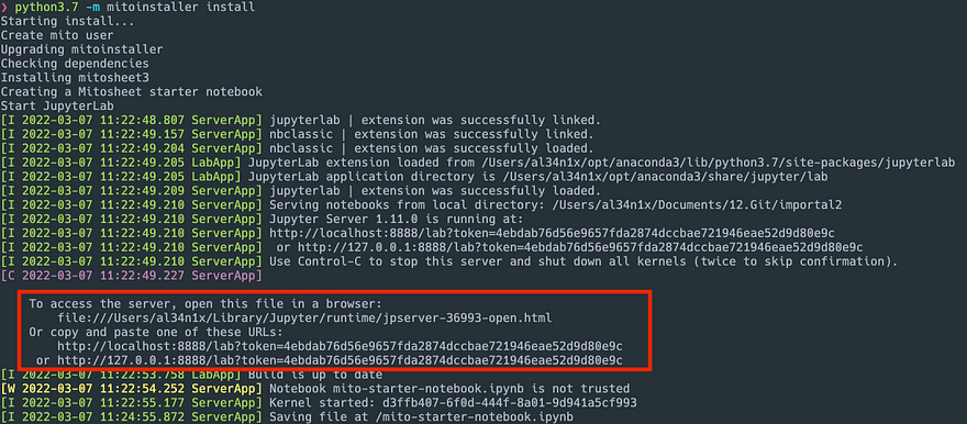

At this point, you should see a new browser or tab opened with Jupyter notebook running. If you find any issue during the installation process, please refer to Mitosheet troubleshooting guide.

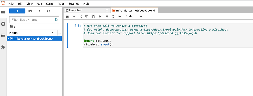
With our notebook up and running, let’s first import some real data. Download the current data-covid-vaccination-eu-eea which includes the European current vaccination status by reporting country.

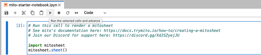
With the first block of code selected, click run.

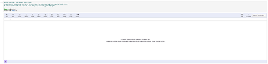
Now, we should be able to see Mito’s interface in action. Click the + option located at the bottom to add some data.

Once the Import Files panel is open, navigate to the file that you have previously downloaded and click on Select a File to Import option.

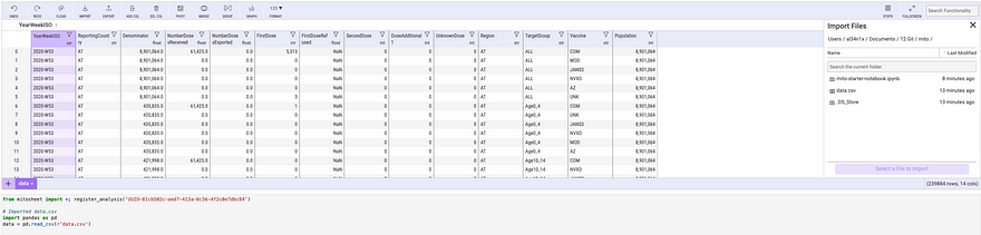
By using MitoSheet you can get the set of Pandas’ instructions required to import and transform data as you move forward with your data analysis without even code.

This is similar to what we did in our previous example in Colab when loading the california_housing_train.csv dataset.

Data Transformation

As part of any data analysis, you might want to filter and sort data. With Mitosheet, you can get this done with a few clicks. Let’s filter the dataset by the ReportingCountry column. I will choose ES (Spain) for the purpose of this example.

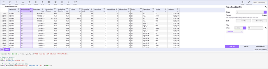
The code keeps evolving as we move forward with the data analysis. This helps you to easily build your notebook and share your results without worrying about coding at all.

We can create pivot tables with a few clicks as well, similar to what you do in Microsoft Excel.

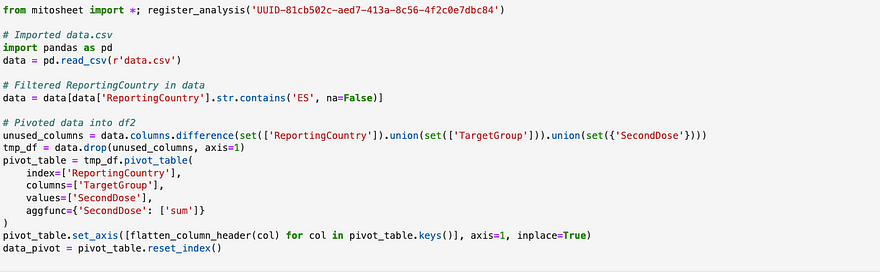
Click the Pivot option on the top menu and select the fields that you will be using as part of the analysis. For this example, I’m reviewing the second dose applied by the target group in Spain.

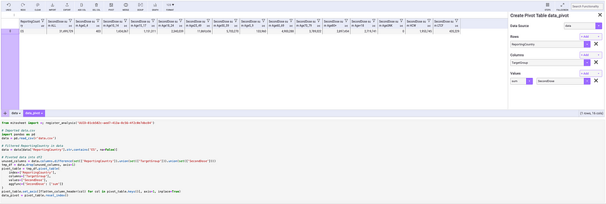
You can see the Pandas’ instructions below.

You want to plot the data, no worries, I got you! Just click the Graph option on the top menu, and select the chart type, X, and Y-Axis value, and you are ok to go.

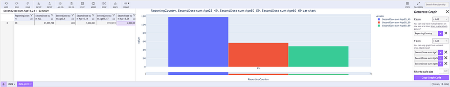
Easy, right? Mitosheet allows you to explore and plot your data without the stress of writing complex code.

Testing Mitosheet Code in Colab

Picture this. Your manager is asking you to share the analysis with your colleagues, but, they use another IDE for data analysis. Let’s test the results in Colab.

Open Colab and load the data-covid-vaccination-eu-eea file. You can drag it and drop it into the sample_data directory.

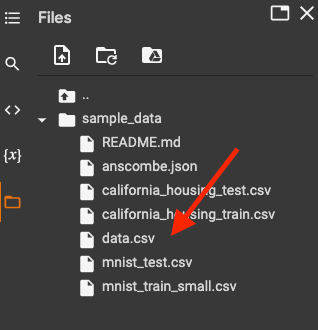
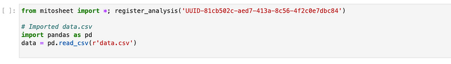
Now, let's leverage the Python code created by MitoSheet. Keep in mind that you need to change the directory reference to ./sample_data/data.csv as highlighted in the pd.read_csv instruction.

# Imported data.csv
import pandas as pd
data = pd.read_csv(r'./sample_data/data.csv')

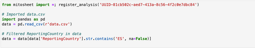
# Filtered ReportingCountry in data
data = data[data['ReportingCountry'].str.contains('ES', na=False)]

# Pivoted data into df2
unused_columns = data.columns.difference(set(['ReportingCountry']).union(set(['TargetGroup'])).union(set({'SecondDose'})))

tmp_df = data.drop(unused_columns, axis=1)

pivot_table = tmp_df.pivot_table( index=['ReportingCountry'], columns=['TargetGroup'], values=['SecondDose'], aggfunc={'SecondDose': ['sum']})

And let’s see the results.

```

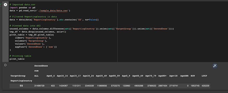
The code actually works! You can easily share the results with your colleagues regardless of the IDE or notebook of their choice.

Summary

MitoSheet allows you to easily explore and transform data without coding by providing a user-friendly interface while reducing the time required to program and debug Python code and focusing on the data analysis itself.

There are plenty of tools that can help you to explore data without being a Python programmer, but, keep in mind that as you dig into the “Data Science rabbit hole”, you might want to get further involved in Python programming to take your Data Scientists skills to a whole new level.

For further information on how to install and work with Mitosheet, please refer to MitoSheet Documentation.

Hope you have found this post informative. Feel free to share it, we want to reach as many people as we can because knowledge must be shared, right?

If you reach this point, Thank you!

<AL34N!X>